Introduction to explainy - black-box model explanations for humans

In this notebook, we will go over the main algorithms of the explainy package.

import pandas as pd
from sklearn.datasets import load_diabetes
from sklearn.ensemble import RandomForestRegressor
from sklearn.model_selection import train_test_split

Installing Explainy

We recommend using some virtual environment. Then there are mainly two ways.

With pip:

pip install explainy

%%capture
!pip install explainy --upgrade

import explainy

print(explainy.__version__)

0.2.8

explainy allows you to create machine learning model explanations based on four different explanation characteristics:

• global: explanation of system functionality

• local: explanation of decision rationale

• contrastive: tracing of decision path

• non-contrastive: parameter weighting

The explanations algorithms in explainy can be categorized as follows:

	non-contrastive	contrastive
global	Permutation Feature Importance	Surrogate Model
local	Shap Values	Counterfactual Example

%load_ext autoreload
%autoreload 2
%matplotlib inline

diabetes = load_diabetes()

X_train, X_test, y_train, y_test = train_test_split(
    diabetes.data, diabetes.target, random_state=0
)
X_test = pd.DataFrame(X_test, columns=diabetes.feature_names)
y_test = pd.DataFrame(y_test)

model = RandomForestRegressor(random_state=0).fit(X_train, y_train)

from explainy.explanations import PermutationExplanation

number_of_features = 4
sample_index = 1

explainer = PermutationExplanation(X_test, y_test, model, number_of_features)
explanation = explainer.explain(sample_index)
print(explanation)
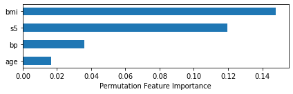
explainer.plot(kind="bar")

The RandomForestRegressor used 10 features to produce the predictions. The prediction of this sample was 251.6.
The feature importance was calculated using the Permutation Feature Importance method.
The four features which were most important for the predictions were: 'bmi' (0.15), 's5' (0.12), 'bp' (0.04), and 'age' (0.02).

explainer.plot(kind="box")

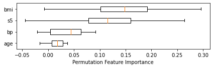
Generate explanations with multiple numbers of features to explain the outcoume. Since the PermuationExplanation method is a global explaination method, all samples will have the same feature importance explanation.

# Global, Non-contrastive
sample_index = 0
for number_of_features in [3, 6, 9]:
    explainer = PermutationExplanation(X_test, y_test, model, number_of_features)
    explanation = explainer.explain(sample_index)
    explainer.plot(kind="box")
    print(explanation)
    print("\n" * 2)

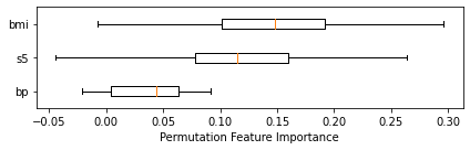
The RandomForestRegressor used 10 features to produce the predictions. The prediction of this sample was 250.6.
The feature importance was calculated using the Permutation Feature Importance method.
The three features which were most important for the predictions were: 'bmi' (0.15), 's5' (0.12), and 'bp' (0.04).

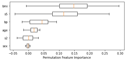
The RandomForestRegressor used 10 features to produce the predictions. The prediction of this sample was 250.6.
The feature importance was calculated using the Permutation Feature Importance method.
The six features which were most important for the predictions were: 'bmi' (0.15), 's5' (0.12), 'bp' (0.04), 'age' (0.02), 's2' (-0.00), and 'sex' (-0.00).

The RandomForestRegressor used 10 features to produce the predictions. The prediction of this sample was 250.6.
The feature importance was calculated using the Permutation Feature Importance method.
The nine features which were most important for the predictions were: 'bmi' (0.15), 's5' (0.12), 'bp' (0.04), 'age' (0.02), 's2' (-0.00), 'sex' (-0.00), 's3' (-0.00), 's1' (-0.01), and 's6' (-0.01).

Let’s use the ShapExplanation to create local explantions for each sample individually.

from explainy.explanations import ShapExplanation

# Local, Non-contrastive
number_of_features = 4
for sample_index in [0, 1, 2]:

    explainer = ShapExplanation(X_test, y_test, model, number_of_features)
    explanation = explainer.explain(sample_index)
    explainer.plot(sample_index)
    print(explanation)
    print("\n" * 2)

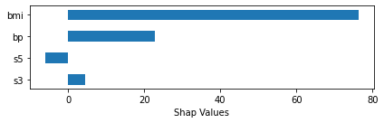
The RandomForestRegressor used 10 features to produce the predictions. The prediction of this sample was 250.6.
The feature importance was calculated using the SHAP method.
The four features which contributed most to the prediction of this particular sample were: 'bmi' (76.30), 'bp' (22.85), 's5' (-5.94), and 's3' (4.48).

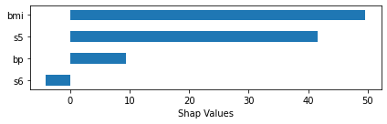
The RandomForestRegressor used 10 features to produce the predictions. The prediction of this sample was 251.6.
The feature importance was calculated using the SHAP method.
The four features which contributed most to the prediction of this particular sample were: 'bmi' (49.60), 's5' (41.64), 'bp' (9.31), and 's6' (-4.04).

The RandomForestRegressor used 10 features to produce the predictions. The prediction of this sample was 169.2.
The feature importance was calculated using the SHAP method.
The four features which contributed most to the prediction of this particular sample were: 'bmi' (22.48), 's5' (-11.53), 'bp' (9.70), and 's6' (-7.94).

Let’s use the SurrogateModelExplanation to create global explantions.

from explainy.explanations import SurrogateModelExplanation

# Global, Contrastive
list_number_of_features = [2, 4]
sample_index = 0
for number_of_features in list_number_of_features:

    explainer = SurrogateModelExplanation(X_test, y_test, model, number_of_features)
    explanation = explainer.explain(sample_index)
    explainer.plot(sample_index)

    print(explanation)
    print("\n" * 2)

Surrogate Model score (coefficient of determination of the prediction): 0.53

Surrogate Model score (coefficient of determination of the prediction): 0.78

The RandomForestRegressor used 10 features to produce the predictions. The prediction of this sample was 250.6.
The feature importance was calculated using a DecisionTreeRegressor surrogate model. Two tree nodes are shown.
The following thresholds were important for the predictions:
The sample has a value of 127.70 if 's5' was less or equal than 0.03.
The sample has a value of 214.95 if 's5' was greater than 0.03.

The RandomForestRegressor used 10 features to produce the predictions. The prediction of this sample was 250.6.
The feature importance was calculated using a DecisionTreeRegressor surrogate model. Four tree nodes are shown.
The following thresholds were important for the predictions:
The sample has a value of 109.80 if 's5' was less or equal than 0.03, and 'bmi' was less or equal than 0.01.
The sample has a value of 165.84 if 's5' was less or equal than 0.03, and 'bmi' was greater than 0.01.
The sample has a value of 171.55 if 's5' was greater than 0.03, and 'bmi' was less or equal than 0.01.
The sample has a value of 239.26 if 's5' was greater than 0.03, and 'bmi' was greater than 0.01.

Let’s use the CounterfactualExplanation to create local explantions and show, how the feature would have had to change to achieve a desired y value.

from explainy.explanations import CounterfactualExplanation

# Local, Contrastive
number_of_features = 6
sample_index = 2
for number_of_features in [4, 8]:
    explainer = CounterfactualExplanation(
        X_test,
        y_test,
        model,
        y_desired=180.0,
        number_of_features=number_of_features,
    )
    explanation = explainer.explain(sample_index)
    explainer.plot(sample_index)
    print(explanation)
    print("\n" * 2)

No delta value set, therefore using the value '8.461'
Start to calculate the counterfactual example. This may take a while...
y_counter_factual: 184.50, lambda: 0.01, local_delta: 4.5, random_seed: 0

No delta value set, therefore using the value '8.461'
Start to calculate the counterfactual example. This may take a while...

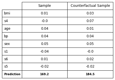
The RandomForestRegressor used 10 features to produce the predictions. The prediction of this sample was 169.2.
The feature importance is shown using a counterfactual example.
The sample would have had the desired prediction of '184.5', if the 'bmi' was '0.03', the 's4' was '0.07', the 'age' was '0.01', and the 'bp' was '0.04'.

y_counter_factual: 184.50, lambda: 0.01, local_delta: 4.5, random_seed: 0

The RandomForestRegressor used 10 features to produce the predictions. The prediction of this sample was 169.2.
The feature importance is shown using a counterfactual example.
The sample would have had the desired prediction of '184.5', if the 'bmi' was '0.03', the 's4' was '0.07', the 'age' was '0.01', the 'bp' was '0.04', the 'sex' was '0.05', the 's1' was '-0.0', the 's6' was '0.02', and the 's5' was '-0.02'.